Fetching Sentinel 2 Data from Sentinel HUB using eo-learn

The open Earth observation (EO) data are accesible via the Copernicus and Landsat programs which large resource for many EO applications, including ocean and land use and land cover monitoring, disaster control, emergency services and humanitarian relief. Given the large amount of high spatial resolution data at high revisit frequency, techniques able to automatically extract complex patterns in such spatio-temporal data are required.

eo-learn is a collection of open source Python packages that have been developed to seamlessly access and process spatio-temporal image sequences acquired by any satellite fleet in a timely and automatic manner. eo-learn is easy to use, it’s design modular, and encourages collaboration – sharing and reusing of specific tasks in a typical EO-value-extraction workflows, such as cloud masking, image co-registration, feature extraction, classification, etc. (info. adopted eo-learn Docs)

eo-learn library acts as a bridge between Earth observation/Remote sensing field and Python ecosystem for data science and machine learning. The library is written in Python and uses NumPy arrays to store and handle remote sensing data. Its aim is to make entry easier for non-experts to the field of remote sensing on one hand and bring the state-of-the-art tools for computer vision, machine learning, and deep learning existing in Python ecosystem to remote sensing experts.(info. adopted eo-learn Docs)

In this post, I would like to use retrieve the time series Sentinel-2 Level-2A for the area in the south of Finland. For this purpose, you need to have an Sentinel Hub account. It is required to create a new configuration (“Add new configuration”) and set the configuration to be based on Python scripts template. After you have prepared a configuration please put configuration’s instance ID into sentinelhub package’s configuration file following the configuration instructions. For Processing API request you also need to obtain and set your oauth client id and secret.

Set up the Configuration

%reload_ext autoreload
%autoreload 2
%matplotlib inline
!sentinelhub.config --instance_id ''
!sentinelhub.config --sh_client_id ''
!sentinelhub.config --sh_client_secret ''
!sentinelhub.config --show
config = SHConfig()

Import the Required Libraries

# Add generic packages
import os
from matplotlib import dates
from tqdm.notebook import tqdm as tqdm
from pathlib import Path
from mpl_toolkits.axes_grid1 import make_axes_locatable

from shapely.geometry import Polygon, box, shape, mapping
import matplotlib.pyplot as plt
import geopandas as gpd
import pandas as pd
import numpy as np
import overpass

# eo-learn and sentinelhub imports
from eolearn.core import EOTask, EOPatch, LinearWorkflow, FeatureType, OverwritePermission, \
    LoadFromDisk, SaveToDisk, EOExecutor, SaveTask
from eolearn.io import SentinelHubInputTask, SentinelHubDemTask, SentinelHubInputBase, get_available_timestamps,ExportToTiff
from eolearn.mask import AddCloudMaskTask, get_s2_pixel_cloud_detector, AddValidDataMaskTask
from eolearn.geometry import VectorToRaster, PointSamplingTask, ErosionTask
from eolearn.features import LinearInterpolation, SimpleFilterTask
from sentinelhub import BBox, CRS, DataSource, MimeType, SentinelHubRequest, SHConfig,BBoxSplitter

Set up the Path to Read & Write data

# Set path to data
data_dir = Path('./data/')
os.listdir(data_dir)

# Folder where data will be stored
OUTPUT_FOLDER = os.path.join('.', 'outputs')
if not os.path.isdir(OUTPUT_FOLDER):
    os.mkdir(OUTPUT_FOLDER)

Read the Area of Interest & Visualize it

# import the country (Finland) & AOI
aoi_filename = data_dir/'aoi_poly.geojson'
country_filename = data_dir/'finland.geojson'
aoi = gpd.read_file(str(aoi_filename))
country = gpd.read_file(str(country_filename))

fig, ax = plt.subplots()
aoi.plot(ax=ax,facecolor='w',edgecolor='r',alpha=0.5)
country.plot(ax=ax, facecolor='w',edgecolor='b',alpha=0.5)
plt.show()

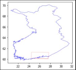
Fig. 1: The AOI in the south of Finland

Change the Projection from WGS84 to UTM

country_crs = CRS.UTM_35N
country = country.to_crs(crs=CRS.ogc_string(country_crs))
aoi = aoi.to_crs(crs=CRS.ogc_string(country_crs))
country.crs

Split to Smaller Tiles

A 3x3 EOPatch sample, where each EOPatch has around 3.30 x 3.30 km (~300 MB per EOPatch), is presented.

aoi_shape = aoi.geometry.values[-1]
width_pix = int((aoi_shape.bounds[2]-aoi_shape.bounds[0]))
height_pix = int((aoi_shape.bounds[3]-aoi_shape.bounds[1]))
print('Dimension of the area is {} x {} m2'.format(width_pix, height_pix))

Create the splitter to obtain a list of bboxes

bbox_splitter = BBoxSplitter([aoi_shape], country_crs, (18 * 3, 13 * 3))

bbox_list = np.array(bbox_splitter.get_bbox_list())
info_list = np.array(bbox_splitter.get_info_list())

Save & Plot the Created Grids (Patches)

# Save grided AOI to the Shapefile
geometry = [Polygon(bbox.get_polygon()) for bbox in bbox_splitter.bbox_list]
idxs_x = [info['index_x'] for info in bbox_splitter.info_list]
idxs_y = [info['index_y'] for info in bbox_splitter.info_list]

df = pd.DataFrame({'index_x':idxs_x, 'index_y':idxs_y})
gdf_all_aoi = gpd.GeoDataFrame(df, crs=CRS.ogc_string(bbox_splitter.bbox_list[0].crs), geometry=geometry)

# save to shapefile
shapefile_name = os.path.join(OUTPUT_FOLDER,'finland_aoi.geojson')
gdf_all_aoi.to_file(shapefile_name, driver='GeoJSON')

# Plot the Grided AOI
fig, ax = plt.subplots()
gdf_all_aoi.plot(ax=ax,facecolor='w', edgecolor='b', alpha=0.5, linewidth=2.5)
plt.show()

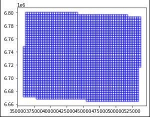
Fig. 1: Created grids (patches) of the AOI

Choose a 3x3 area

Finding the Centeral Patch

clm_x = gdf_all_aoi[gdf_all_aoi['index_x'] == 35]
clm_x[clm_x['index_y'] == 25]

Select 9 patches & save them to disk

# Select a central patch
ID = 1330 

# Obtain surrounding patches
patchIDs = []
for idx, [bbox, info] in enumerate(zip(bbox_list, info_list)):
    if (abs(info['index_x'] - info_list[ID]['index_x']) <= 1 and
        abs(info['index_y'] - info_list[ID]['index_y']) <= 1):
        patchIDs.append(idx)
        
# Change the order of the patches (used for plotting later)
patchIDs = np.transpose(np.fliplr(np.array(patchIDs).reshape(3, 3))).ravel()

    
# Prepare info of selected EOPatches
geometry = [Polygon(bbox.get_polygon()) for bbox in bbox_list[patchIDs]]
idxs_x = [info['index_x'] for info in info_list[patchIDs]]
idxs_y = [info['index_y'] for info in info_list[patchIDs]]

gdf_sellected_area = gpd.GeoDataFrame({'index_x': idxs_x, 'index_y': idxs_y}, 
                       crs= CRS.ogc_string(country_crs), 
                       geometry=geometry)

# save to shapefile
shapefile_name = os.path.join(OUTPUT_FOLDER,'selected_3x3_finland.geojson')
gdf_sellected_area.to_file(shapefile_name,driver='GeoJSON')

Visualize the selected patches

poly = gdf_sellected_area['geometry'][0]
x1, y1, x2, y2 = poly.bounds
aspect_ratio = (y1 - y2) / (x1 - x2)

# content of the geopandas dataframe
gdf_sellected_area.head()

fontdict = {'family': 'monospace', 'weight': 'normal', 'size': 6}
# if bboxes have all same size, estimate offset
xl, yl, xu, yu = gdf_sellected_area.geometry[0].bounds
xoff, yoff = (xu-xl)/3, (yu-yl)/5
# figure
fig, ax = plt.subplots(figsize=(10,10))
gdf_all_aoi.plot(ax=ax, facecolor='w', edgecolor='b', alpha=0.5, linewidth=2.5)
gdf_sellected_area.plot(ax=ax, facecolor='w', edgecolor='r', alpha=0.5, linewidth=2)
ax.set_title('Finland AOI tiled in a 18 x 13 grid');

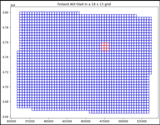
Fig. 1: selected 3 * 3 patches (red)

Define WorkFlow Tasks

Read 6 bands of S2L2A with 10% cloud coverage from Sentinel HUB

# add a request for B(B02), G(B03), R(B04), NIR (B08), SWIR1(B11), SWIR2(B12) 
custom_script = ['B02', 'B03', 'B04', 'B08', 'B11', 'B12']
add_data = SentinelHubInputTask(
    data_source = DataSource.SENTINEL2_L2A, 
    bands_feature =(FeatureType.DATA, 'BANDS'), # save under name 'BANDS'
    bands =custom_script, # custom url for 6 specific bands
    resolution = 10, # resolution x, y
    maxcc = 0.1, # maximum allowed cloud cover of original ESA tiles
    config =config
)

# TASK FOR SAVING TO OUTPUT (if needed)
path_out = os.path.join('.', 'outputs', 'eopatches_small')
if not os.path.isdir(path_out):
    os.makedirs(path_out)
save = SaveTask(path=path_out, overwrite_permission=2, compress_level=1)

Define & Execute the Workflow

# Define the workflow
workflow = LinearWorkflow(
    add_data,
    save
)    
    
# Execute the workflow
time_interval = ['2017-01-01', '2017-12-31'] # time interval for the SH request

# define additional parameters of the workflow
execution_args = []
for idx, bbox in enumerate(bbox_list[patchIDs]):
    execution_args.append({
        add_data:{'bbox': bbox, 'time_interval': time_interval},
        save: {'eopatch_folder': 'eopatch_{}'.format(idx)}
    })
    
executor = EOExecutor(workflow, execution_args, save_logs=True, logs_folder=OUTPUT_FOLDER)
executor.run(workers=5, multiprocess=False)

executor.make_report()

Select the Median image between time series data

# Draw the RGB image
path_out = os.path.join('.', 'outputs', 'eopatches_small')
fig = plt.figure(figsize=(20, 20 * aspect_ratio))


for i in tqdm(range(len(patchIDs))):
    eopatch = EOPatch.load('{}/eopatch_{}'.format(path_out, i), lazy_loading=True)
    ax = plt.subplot(3, 3, i + 1)
    plt.imshow(np.median(eopatch.data['BANDS'][..., [2, 1, 0]], axis=0).squeeze())
    plt.xticks([])
    plt.yticks([])
    ax.set_aspect("auto")
    del eopatch

fig.subplots_adjust(wspace=0, hspace=0)

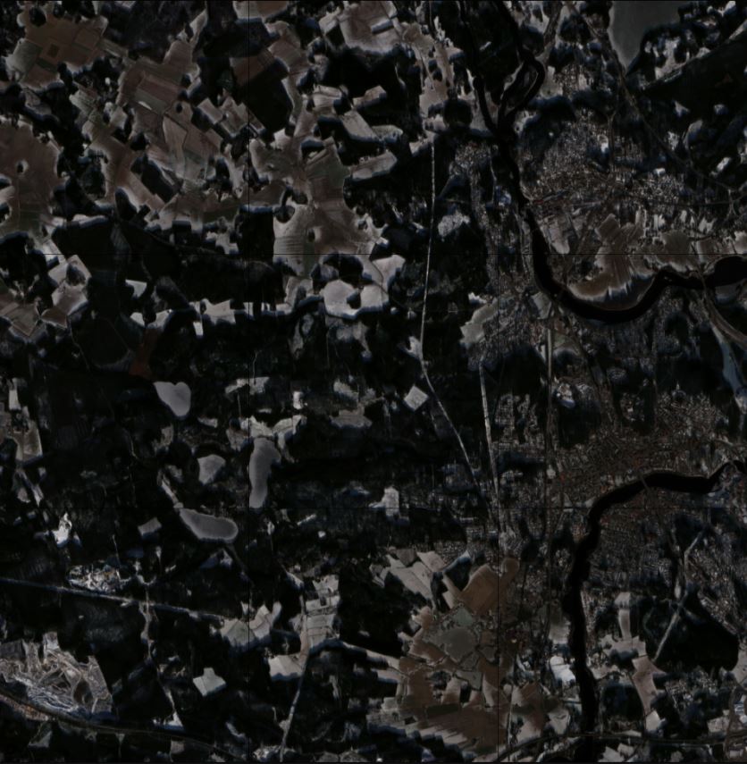
Fig. 1: Visualization selected image for each patch

Source:

Behzad Valipour Sh.